import rmm
import cupy as cp
from rmm.allocators.cupy import rmm_cupy_allocator

rmm.reinitialize(managed_memory=False, pool_allocator=True)
cp.cuda.set_allocator(rmm_cupy_allocator)1 Key concepts of Dask library
Dask is a Python library for parallel and distributed computing.
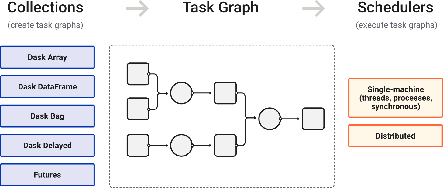
Dask is lazily evaluated. The result from a computation is not computed until you ask for it (call .compute()). Instead, a Dask task graph for the computation is produced.
在调用 .compute() 后,Dask schedulers 依据 task graph 自动调度与执行任务(顺行或并行)。
针对大数据集:
选择合适的数据结构(支持分块)和算法。
选择合适的文件格式(支持并行 IO),如 ZARR。
2 Memory management
- If your data fits in GPU VRAM, use the pool allocator for speed.
- If your data is larger than VRAM, use managed memory to spill to host RAM.
import rmm
import cupy as cp
from rmm.allocators.cupy import rmm_cupy_allocator

rmm.reinitialize(managed_memory=True, pool_allocator=False)
cp.cuda.set_allocator(rmm_cupy_allocator)
3 Setup of the AnnData object
import os
import anndata as ad
import wget
import scanpy as sc
# cancel all proxies
proxies = [
"HTTP_PROXY",
"HTTPS_PROXY",
"http_proxy",
"https_proxy",
"ALL_PROXY",
"all_proxy",
"SOCKS_PROXY",
"socks_proxy",
]
for key in proxies:
os.environ.pop(key, None)work_dir = "/home/yangrui/test/data"
os.chdir(work_dir)wget.download("https://figshare.com/ndownloader/files/45788454", out="adata.raw.h5ad")
wget.download(
"https://scverse-exampledata.s3.eu-west-1.amazonaws.com/rapids-singlecell/dli_census.h5ad",
out="dli_census.h5ad",
)
wget.download(
"https://scverse-exampledata.s3.eu-west-1.amazonaws.com/rapids-singlecell/1M_brain_cells_10X.sparse.h5ad",
out="nvidia_1.3M.h5ad",
)
wget.download(
"https://datasets.cellxgene.cziscience.com/3817734b-0f82-433b-8c38-55b214200fff.h5ad",
out="cell_atlas.h5ad",
)对于大数据集,推荐利用 ZARR 格式分块存储,从而实现按需读取,节约内存。
# read an element from a store lazily
from anndata.experimental import read_elem_lazy as read_dask
import h5py
SPARSE_CHUNK_SIZE = 20000
data_file = "nvidia_1.3M.h5ad"
f = h5py.File(data_file)
X = f["X"]
shape = X.attrs["shape"]
adata = ad.AnnData(
# 设置每一个数据块的维度
# (细胞维度,基因维度)
# CSR sparse:(SPARSE_CHUNK_SIZE, shape[1])。按行读取,即按行(细胞维度)切割数据,对于每一行,必须保持基因维度完整(即第二维度必须等于总列数)
# CSC sparse:(shape[0], SPARSE_CHUNK_SIZE)。按列读取,即按列(基因维度)切割数据,对于每一列,必须保持细胞维度完整(即第一维度必须等于总行数)
X=read_dask(X, (SPARSE_CHUNK_SIZE, shape[1])),
obs=ad.io.read_elem(f["obs"]),
var=ad.io.read_elem(f["var"]),
)
f.close()
# 写为 ZARR 格式,其将每一个块存储为一个独立的文件,具有更加优异的并行 IO 性能
# HDF5 虽也支持分块,但性能远不如 ZARR
adata.write_zarr("nvidia_1.3M.zarr")from anndata.experimental import read_elem_lazy as read_dask
import h5py
SPARSE_CHUNK_SIZE = 20000
data_file = "cell_atlas.h5ad"
f = h5py.File(data_file)
X = f["X"]
shape = X.attrs["shape"]
adata = ad.AnnData(
X=read_dask(X, (SPARSE_CHUNK_SIZE, shape[1])),
obs=ad.io.read_elem(f["obs"]),
var=ad.io.read_elem(f["var"]),
)
f.close()
adata.write_zarr("cell_atlas.zarr")4 Basic demo workflow of rapids-singlecell
import scanpy as sc
import anndata as ad
import rapids_singlecell as rsc
import warnings
warnings.filterwarnings("ignore")
import rmm
import cupy as cp
from rmm.allocators.cupy import rmm_cupy_allocator
# use pool allocator for small datasets
# use managed memory for large datasets
rmm.reinitialize(managed_memory=True, pool_allocator=False, devices=[0, 1])
cp.cuda.set_allocator(rmm_cupy_allocator)4.1 Load and prepare data
work_dir = "/home/yangrui/test/data"
os.chdir(work_dir)
adata_file = "dli_census.h5ad"adata = sc.read_h5ad(adata_file)Note: Load data into GPU memory!
# load data into GPU memory
rsc.get.anndata_to_GPU(adata)
4.2 Preprocessing
4.2.1 Quality control
Calculate QC metrics:
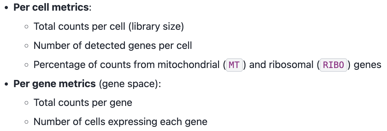
rsc.pp.flag_gene_family(adata, gene_family_name="MT", gene_family_prefix="MT")rsc.pp.flag_gene_family(adata, gene_family_name="RIBO", gene_family_prefix="RPS")rsc.pp.calculate_qc_metrics(adata, qc_vars=["MT", "RIBO"])Visualize QC metrics:
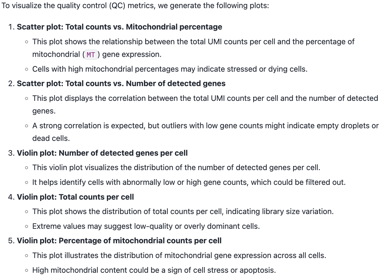
sc.pl.scatter(adata, x="total_counts", y="pct_counts_MT")
sc.pl.scatter(adata, x="total_counts", y="n_genes_by_counts")
sc.pl.violin(adata, "n_genes_by_counts", jitter=0.4, groupby="assay")
sc.pl.violin(adata, "total_counts", jitter=0.4, groupby="assay")
sc.pl.violin(adata, "pct_counts_MT", jitter=0.4, groupby="assay")4.2.2 Filtering
adata = adata[adata.obs["n_genes_by_counts"] > 500]
adata = adata[adata.obs["n_genes_by_counts"] < 5000]
adata = adata[adata.obs["pct_counts_MT"] < 20]
rsc.pp.filter_genes(adata, min_cells=3)4.2.3 Normalization
adata.layers["counts"] = adata.X.copy()
rsc.pp.normalize_total(adata, target_sum=1e4)
rsc.pp.log1p(adata)
4.2.4 Select highly variable genes
rsc.pp.highly_variable_genes(adata, n_top_genes=5000, flavor="seurat_v3", layer="counts", batch_key="assay")sc.pl.highly_variable_genes(adata, log=True)adata.raw = adataWe now restrict our AnnData object to only the highly variable genes. This step reduces the number of features, focusing the analysis on the most informative genes while improving computational efficiency.
rsc.pp.filter_highly_variable(adata)As in Scanpy, you can regress out any numerical column from .obs, allowing for the correction of batch effects, sequencing depth, or other confounding factors.
rsc.pp.regress_out(adata, keys=["total_counts", "pct_counts_MT"])4.2.5 Scale
Finally, we scale the count matrix to obtain a z-score transformation, standardizing gene expression across cells.
To prevent extreme values from dominating the analysis, we apply a cutoff of 10 standard deviations.
This ensures that highly expressed genes do not disproportionately influence downstream computations.
rsc.pp.scale(adata, max_value=10)4.3 Clustering and visualization
4.3.1 PCA
rsc.tl.pca(adata, n_comps=100)sc.set_figure_params(figsize=(22, 8))
sc.pl.pca_variance_ratio(adata, log=True, n_pcs=100)
sc.set_figure_params(figsize=(10, 10))Note: unload data from GPU memory!
rsc.get.anndata_to_CPU(adata)4.3.2 Compute the neighborhood graph and UMAP
# n_neighbors: The size of local neighborhood.
# Larger values result in more global views of the manifold, while smaller values result in more local data being preserved. In general, values should be in the range 2 to 100.

# algorithm:
# Exact nearest neighbor search:
# - 'brute'
# Approximate nearest neighbor search:
# - 'ivfflat': suitable for large datasets.
# - 'ivfpq': a variant of 'ivfflat' that compresses data for more efficient memory usage, trading off some accuracy.
# 'cagra': optimized for fast, high-accuracy queries on GPUs.
# 'nn_descent': incrementally refines the nearest neighbor search and works well for large, high-dimensional datasets.
rsc.pp.neighbors(adata, n_neighbors=15, n_pcs=40, algorithm="brute", use_rep="X_pca")
UMAP preserves local and global structure in the data.
rsc.tl.umap(adata)4.3.3 Clustering
rsc.tl.louvain(adata, resolution=0.6, key_added="louvain")# An improved version of Louvain that guarantees well-connected, more stable clusters.
rsc.tl.leiden(adata, resolution=0.6, key_added="leiden")sc.pl.umap(adata, color=["louvain", "leiden"], legend_loc="on data")sc.pl.umap(adata, color=["cell_type", "assay"],ncols=1)4.3.4 Batch correction
Harmony works by adjusting the PCs, so this function should be run after PCA but before computing the neighbor graph.
# in general, using float32 is enough
rsc.pp.harmony_integrate(
    adata, key="assay", dtype=cp.float32, basis="X_pca", adjusted_basis="X_pca_harmony"
)
Re-run neighborhood search, UMAP, and graph-based clustering with the corrected PCs!
rsc.pp.neighbors(
    adata, n_neighbors=15, n_pcs=40, use_rep="X_pca_harmony", key_added="harmony"
)

rsc.tl.umap(adata, neighbors_key="harmony", key_added="X_umap_harmony")

rsc.tl.louvain(
    adata, resolution=0.6, neighbors_key="harmony", key_added="louvain_harmony"
)

rsc.tl.leiden(
    adata, resolution=0.6, neighbors_key="harmony", key_added="leiden_harmony"
)
sc.pl.embedding(
adata,
basis="X_umap_harmony",
color=["louvain_harmony", "leiden_harmony"],
legend_loc="on data",
)sc.pl.embedding(adata, basis="X_umap_harmony", color=["cell_type", "assay"], ncols=1)4.3.5 T-SNE
t-SNE preserves local structure and reveals complex patterns in the data.
rsc.tl.tsne(
    adata,
    n_pcs=40,
    perplexity=30,
    early_exaggeration=12,
    learning_rate=200,
    use_rep="X_pca_harmony",
)
sc.pl.tsne(adata, color=["cell_type", "assay"], ncols=1)4.4 Differential expression analysis
传统方法(如 Wilcoxon)关注的是:基因 A 在组 1 和组 2 之间的表达分布是否有差异。
逻辑回归关注的是:仅凭基因 A 的表达量,我有多大把握将一个细胞准确归类到目标类群?其同时考虑所有基因。
rsc.tl.rank_genes_groups_logreg(adata, groupby="cell_type", use_raw=False)sc.pl.rank_genes_groups(adata)4.5 Diffusion map embedding
A non-linear dimensionality reduction method that preserves continuous structure of the data, suitable for capturing trajectory-like relationships in single-cell data.
rsc.tl.diffmap(adata, neighbors_key="harmony")

# Due to an issue with plotting in Scanpy, we need to shift the first component of the diffusion map by removing the first column
# 平凡解(Trivial Solution):扩散矩阵的第一特征值始终为 1,而其对应的第一特征向量(Eigenvector 0)是一个常数向量(所有元素都相等,或者非常接近)。
# 无信息量:在降维空间中,这个分量代表了数据集的背景或整体连通性,它不包含任何关于细胞异质性、细胞类型或发育轨迹的区分信息。
adata.obsm["X_diffmap"] = adata.obsm["X_diffmap"][:, 1:]
sc.pl.diffmap(adata, color="cell_type")5 Out-of-Core Single-Cell Analysis with Rapids-SingleCell and Dask
By leveraging Dask, we can:
Process large-scale single-cell datasets without exceeding memory limits.
Enable chunk-based execution, loading only the necessary data into memory at any time.
import dask
import gc

from dask_cuda import LocalCUDACluster
from dask.distributed import Client
import rmm
import cupy as cp
from rmm.allocators.cupy import rmm_cupy_allocator5.1 Initializing a Dask Cluster for Out-of-Core Computation
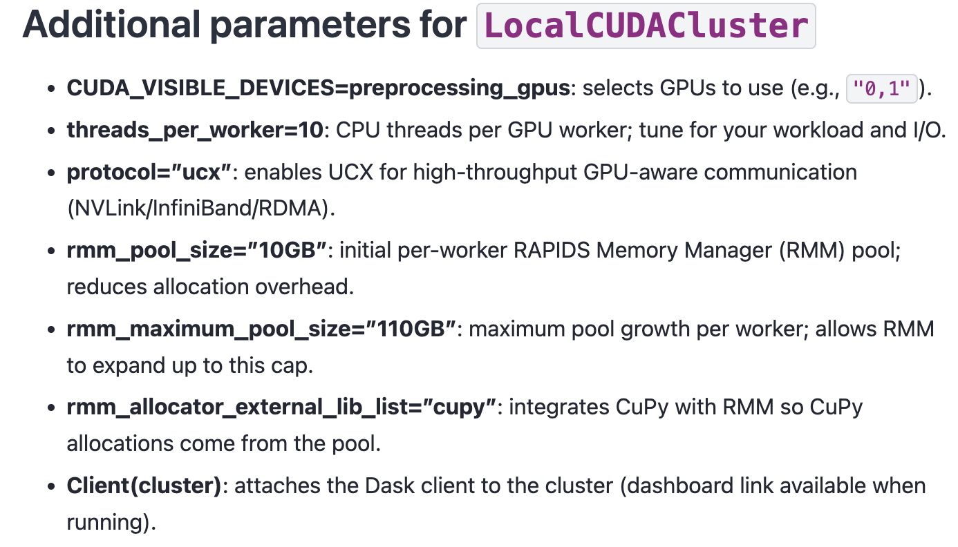
cluster = LocalCUDACluster(
CUDA_VISIBLE_DEVICES="0,1",
threads_per_worker=32,
protocol="ucx",
rmm_pool_size="10GB",
rmm_maximum_pool_size="20GB",
rmm_allocator_external_lib_list="cupy",
)
client = Client(cluster)
clientYou’d better run those code in the following way:
To reduce the chance of OOM, set a lower value for SPARSE_CHUNK_SIZE.
# %%
import os
# %%
work_dir = "/home/yangrui/test/data"
os.chdir(work_dir)
# %%
import dask
import gc
from dask_cuda import LocalCUDACluster
from dask.distributed import Client
# %%
import rmm
import cupy as cp
from rmm.allocators.cupy import rmm_cupy_allocator
# %% Initialize a Dask Cluster for Out-of-Core Computation
# MANDATORY: THE 'if __name__ == "__main__":' PROTECTION
# Why this is necessary:
# 1. Spawn Method: When using GPUs, Dask uses the 'spawn' start method
# to create worker processes.
# 2. Resource Duplication: Unlike 'fork', 'spawn' starts a fresh Python process
# that re-imports the entire script to initialize the environment.
# 3. Recursive Trap: Without this check, every child worker would attempt to
# initialize its own Dask cluster upon import, leading to an infinite
# loop of process creation (a "fork bomb") and immediate system failure.
# 4. Entry Point: This block ensures the cluster and client are only created
# once in the parent process, providing a safe entry point for execution.
if __name__ == "__main__":
cluster = LocalCUDACluster(
CUDA_VISIBLE_DEVICES="0,1",
threads_per_worker=32,
protocol="ucx",
rmm_pool_size="12GB",
rmm_maximum_pool_size="22GB",
rmm_allocator_external_lib_list="cupy",
)
client = Client(cluster)
print(client)
# %%
import rapids_singlecell as rsc
import scanpy as sc
import anndata as ad
# %% Load Large Datasets into AnnData with Dask
import zarr
from anndata.experimental import read_elem_lazy as read_dask
SPARSE_CHUNK_SIZE = 20000
data_file = "nvidia_1.3M.zarr"
f = zarr.open(data_file)
X = f["X"]
shape = X.attrs["shape"]
adata = ad.AnnData(
X=read_dask(X, (SPARSE_CHUNK_SIZE, shape[1])),
obs=ad.io.read_elem(f["obs"]),
var=ad.io.read_elem(f["var"]),
)
# %% Transfer AnnData to GPU for Accelerated Computation
rsc.get.anndata_to_GPU(adata)6 Multi-GPU Showcase with persist
By leveraging Dask and RAPIDS, we can:
Process massive single-cell datasets without exceeding memory limits.
Fully utilize all available GPUs, scaling performance across multiple devices.
Enable chunk-based execution, efficiently managing memory by loading only necessary data.