Bulk RNA-seq pseudotime analysis

1 Introduction

In scRNA-seq, various tools, such as Monocle3, provide the capability of performing pseudotime analysis. In brief, assume that there are both progenitors and more differentiated progenies in an scRNA-seq dataset. If we consider the most undeferentiated progenitors as the developmental origin (assigning them the number \(0\)), and the most differentiated progenies the developmental ends (assigning them the number 10), then we can assign each intermediate cell within them a number between \(0\) and \(10\). For cells with numbers approaching \(0\) more, they are more similar with the progenitors in terms of their RNA expression patterns and vice versa. Once we assign each cell a number (i.e. a developmental pseudotime point) and order them based on their pseudotime, we can arrange highly variable genes based on their peaking expression patterns (i.e. genes with peaking expression patterns at early stages are placed at the left, etc.).

In bulk RNA-seq, the number of samples is far less than the number of cells in scRNA-seq, where each cell can be regarded as a sample, so the gene expression dynamics along the developmental stages are not so smooth (i.e. jagged) as we have seen in scRNA-seq if we do the same analysis in bulk RNA-seq as in scRNA-seq. Therefore, to make the gene expression dynamics smoother along the developmental stages, we need to obtain more pseudo/interpolated time points than those we have.

Briefly, to achieve this goal, we need to do the following things:

Define the time scale among developmental samples based on their mutual Euclidean distances calculated from their coordinates (Dim.1, Dim.2) obtained from their PCA space (i.e. consider the earliest sample as the developmental origin, assign it \(0\), and for the remaining samples, use their Euclidean disntances accumulated from the origin as their developmental time points).
Scale the time scale to (0, 10).
Fit a spline for each gene based its \((time, expression)\) pairs along the actual developmental stages, and use this fitted spline to interpolate more \((time, expression)\) pairs (using the loess method in modelr package).
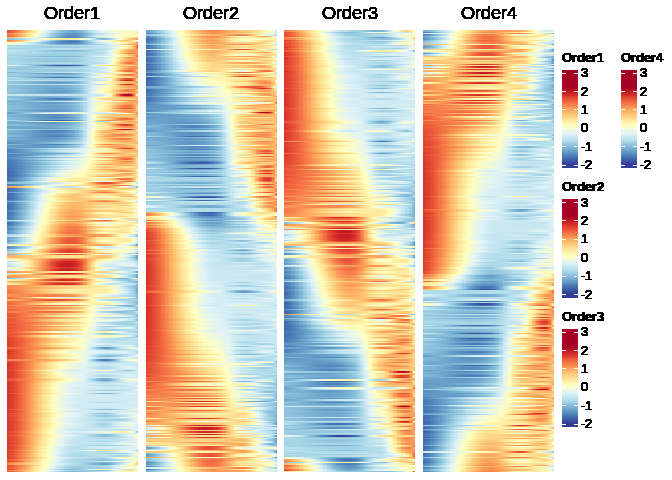
For each gene, obtain its PCA coordinate (Dim.1, Dim.2), and then feed all possible signed combinations of Dim.1 and Dim.2 of all genes to atan2 to get a sequence of values used to sort genes.
Visualize gene expression dynamics along interpolated time points to pick the expected one.

2 Pipeline

suppressWarnings(suppressMessages(library(vroom)))
suppressWarnings(suppressMessages(library(tidyverse)))
suppressWarnings(suppressMessages(library(ggplot2)))
suppressWarnings(suppressMessages(library(ggrepel)))
suppressWarnings(suppressMessages(library(magrittr)))
suppressWarnings(suppressMessages(library(FactoMineR)))
suppressWarnings(suppressMessages(library(ComplexHeatmap)))
suppressWarnings(suppressMessages(library(scales)))
suppressWarnings(suppressMessages(library(modelr)))
suppressWarnings(suppressMessages(library(RColorBrewer)))
suppressWarnings(suppressMessages(library(patchwork)))
suppressWarnings(suppressMessages(library(showtext)))

font_family <- "Arial"

font_df <- filter(font_files(), family == font_family)
font_add(
    family = font_family,
    regular = if ("Regular" %in% font_df[["face"]]) font_df[["file"]][font_df[["face"]] == "Regular"] else stop("no font file found"),
    bold = if ("Bold" %in% font_df[["face"]]) font_df[["file"]][font_df[["face"]] == "Bold"] else NULL,
    italic = if ("Bold Italic" %in% font_df[["face"]]) font_df[["file"]][font_df[["face"]] == "Bold Italic"] else NULL,
    bolditalic = if ("Italic" %in% font_df[["face"]]) font_df[["file"]][font_df[["face"]] == "Italic"] else NULL
)
showtext_auto()

# specify input gene expression matrix
# containing one ID column named "GeneID"
# the remaining columns are sample columns named in the form of "SampleID.Replicate" (e.g. Skin.1, Skin.2, etc.)
# SampleID must not contain "."
# Replicate must be one or more integers
expr_file <- "./data/RNA_TPM.txt"
# specify the sample levels, reflecting their actual developmental stages
sample_dev_order <- c("DAI0", "DAI3", "DAI6", "DAI9", "DAI12")
time_points_num <- 500

expr <- vroom(expr_file) %>%
    as.data.frame() %>%
    set_rownames(.[["GeneID"]]) %>%
    select(-all_of("GeneID")) %>%
    distinct()
sample_df <- strsplit(names(expr), ".", fixed = T) %>%
    do.call(rbind, .) %>%
    as.data.frame() %>%
    set_colnames(c("SampleID", "Replicate")) %>%
    mutate(Sample = paste0(SampleID, ".", Replicate))

# calculate the mean expression value of each gene within each sample
data <- data.frame(GeneID = row.names(expr))
for (id in unique(sample_df[["SampleID"]])) {
    id_reps <- filter(sample_df, SampleID == id) %>%
        pull(Sample) %>%
        unique()
    id_mean_expr <- data.frame(Expr = rowMeans(expr[, id_reps]))
    names(id_mean_expr) <- id
    data <- bind_cols(data, id_mean_expr)
}
data <- as.data.frame(data) %>%
    set_rownames(.[["GeneID"]]) %>%
    select(-all_of("GeneID"))

# use row variances to identify the top 3000 most variable genes
# log2-trsanformation is recommended for reducing variance variation among genes
data <- log2(data + 1)
data[["var"]] <- apply(data, 1, var)
data <- data %>%
    arrange(desc(var)) %>%
    slice_head(n = 3000) %>%
    select(-all_of("var"))
data <- data[, sample_dev_order]

# perform PCA analysis over samples (samples as observations)
# calculate Euclidean distances among samples based on their coordinates (Dim.1, Dim.2) in sample PCA space
# obtain the developmental time scale by accumulating distances of mutual samples
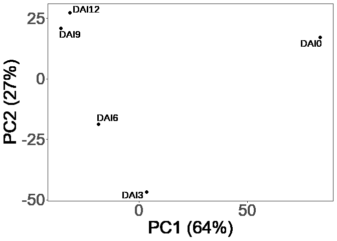
sample_pca <- PCA(t(data), scale.unit = T, ncp = 5, graph = F)
sample_pca_coords <- sample_pca$ind$coord[, 1:2]

# visualize sample positions in PCA space
sample_pca_coords_vis <- as.data.frame(sample_pca_coords)
sample_pca_coords_vis[["Sample"]] <- row.names(sample_pca_coords_vis)
sample_pca_eig_vis <- as.data.frame(sample_pca$eig)

ggplot(sample_pca_coords_vis, aes(Dim.1, Dim.2)) +
    geom_point(size = 2) +
    geom_text_repel(aes(label = Sample), size = 5, min.segment.length = 3) +
    xlab(paste0("PC1 (", round(sample_pca_eig_vis["comp 1", "percentage of variance"]), "%)")) +
    ylab(paste0("PC2 (", round(sample_pca_eig_vis["comp 2", "percentage of variance"]), "%)")) +
    theme_bw() +
    theme(
        panel.grid.major = element_blank(),
        panel.grid.minor = element_blank(),
        axis.title.x = element_text(size = 26),
        axis.title.y = element_text(size = 26),
        axis.text.x = element_text(size = 24),
        axis.text.y = element_text(size = 24),
        legend.text = element_text(size = 24),
        legend.title = element_text(size = 26),
        text = element_text(family = "Arial")
    )

sample_dists <- as.matrix(dist(sample_pca_coords, method = "euclidean"))

# visualize sample distances via heatmap
Heatmap(sample_dists, cluster_rows = F, cluster_columns = F)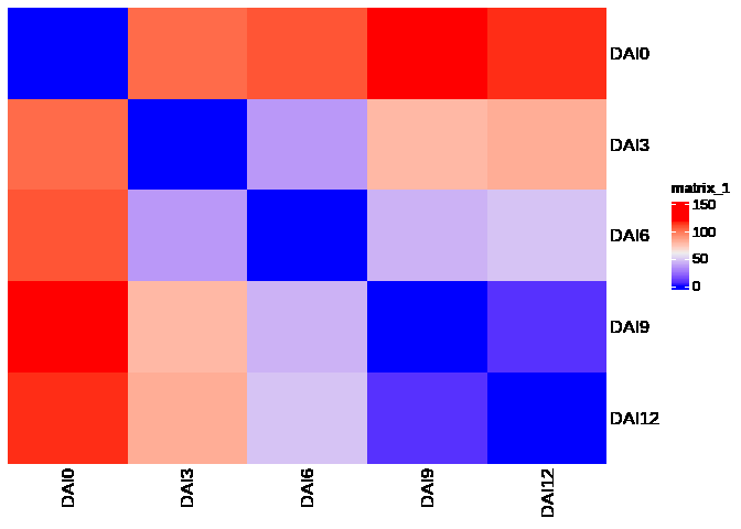

# calculate the developmental time scale by accumulating distances of mutual samples along the actual developmental stages
raw_timeline <- cumsum(c(0, sapply(2:ncol(data), function(x) {
    sample_dists[x - 1, x]
})))
# scale the raw time scale to (0, 10)
new_timeline <- scales::rescale(raw_timeline, to = c(0, 10))

# fit a spline for each gene and obtain 500 time points by interpolation
data_scale <- as.data.frame(t(scale(t(data))))

# interpolate more time points (e.g., 500) to make the expression dynamics smoother along the developmental stages
# based on the fitted spline for each gene (using the loess method in modelr package)
pseudotime_model_fun <- function(sample_value, sample_timeline, time_points_num = 500) {
    grid <- data.frame(time = seq(0, 10, length.out = time_points_num))
    data <- tibble(value = sample_value, time = sample_timeline)
    model <- loess(value ~ time, data)
    predict <- add_predictions(grid, model)
    return(predict)
}

pseudotime_model_res <- apply(data_scale, 1, pseudotime_model_fun, sample_timeline = new_timeline, time_points_num = time_points_num)
res <- lapply(pseudotime_model_res, function(x) {
    x[["pred"]]
}) %>%
    do.call(rbind, .) %>%
    as.data.frame() %>%
    set_colnames(pseudotime_model_res[[1]][["time"]])

# perform PCA analysis over genes
# use atan2 method to sort genes based on their coordinates (Dim.1, Dim.2) in gene PCA space
gene_pca <- PCA(res, scale.unit = T, ncp = 5, graph = F)
gene_pca_coords <- gene_pca$ind$coord[, 1:2]
res <- bind_cols(res, gene_pca_coords)

# we have four signed combinations of Dim.1 and Dim.2
res[["atan2.1"]] <- atan2(res[["Dim.1"]], res[["Dim.2"]])
res[["atan2.2"]] <- atan2(res[["Dim.1"]], -res[["Dim.2"]])
res[["atan2.3"]] <- atan2(-res[["Dim.1"]], res[["Dim.2"]])
res[["atan2.4"]] <- atan2(-res[["Dim.1"]], -res[["Dim.2"]])

# sort genes based on their atan2 values in ascending order
res_order1 <- arrange(res, res[["atan2.1"]])
res_order2 <- arrange(res, res[["atan2.2"]])
res_order3 <- arrange(res, res[["atan2.3"]])
res_order4 <- arrange(res, res[["atan2.4"]])

# pick the expected one
p1 <- Heatmap(as.matrix(res_order1[, 1:time_points_num]),
    cluster_rows = F,
    cluster_columns = F,
    show_row_names = F,
    show_column_names = F,
    column_title = "Order1",
    heatmap_legend_param = list(title = "Order1", legend_height = unit(2, "cm")),
    col = colorRampPalette(rev(brewer.pal(n = 11, name = "RdYlBu")))(100)
)
p2 <- Heatmap(as.matrix(res_order2[, 1:time_points_num]),
    cluster_rows = F,
    cluster_columns = F,
    show_row_names = F,
    show_column_names = F,
    column_title = "Order2",
    heatmap_legend_param = list(title = "Order2", legend_height = unit(2, "cm")),
    col = colorRampPalette(rev(brewer.pal(n = 11, name = "RdYlBu")))(100)
)
p3 <- Heatmap(as.matrix(res_order3[, 1:time_points_num]),
    cluster_rows = F,
    cluster_columns = F,
    show_row_names = F,
    show_column_names = F,
    column_title = "Order3",
    heatmap_legend_param = list(title = "Order3", legend_height = unit(2, "cm")),
    col = colorRampPalette(rev(brewer.pal(n = 11, name = "RdYlBu")))(100)
)
p4 <- Heatmap(as.matrix(res_order4[, 1:time_points_num]),
    cluster_rows = F,
    cluster_columns = F,
    show_row_names = F,
    show_column_names = F,
    column_title = "Order4",
    heatmap_legend_param = list(title = "Order4", legend_height = unit(2, "cm")),
    col = colorRampPalette(rev(brewer.pal(n = 11, name = "RdYlBu")))(100)
)

p1 + p2 + p3 + p4